|
|
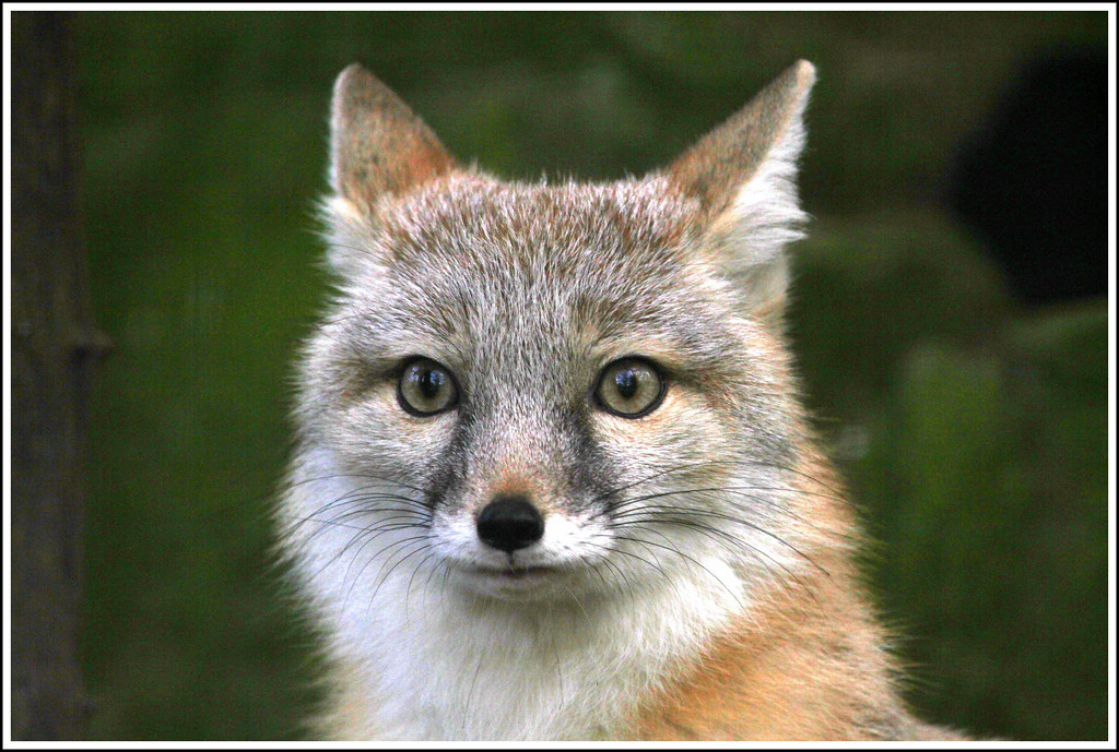
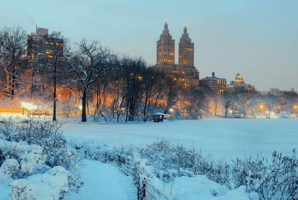
In this project, we use deep learning to generate a neural radiance field or a 3D reconstruction of an object using pictures taken at different angles. By sampling rays in world space from images, sampling points along those rays, and learning the color and opacity of each world-space coordinate, we can mimic the way light diffuses through air to render a 3 dimensional object at any angle.
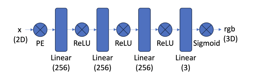
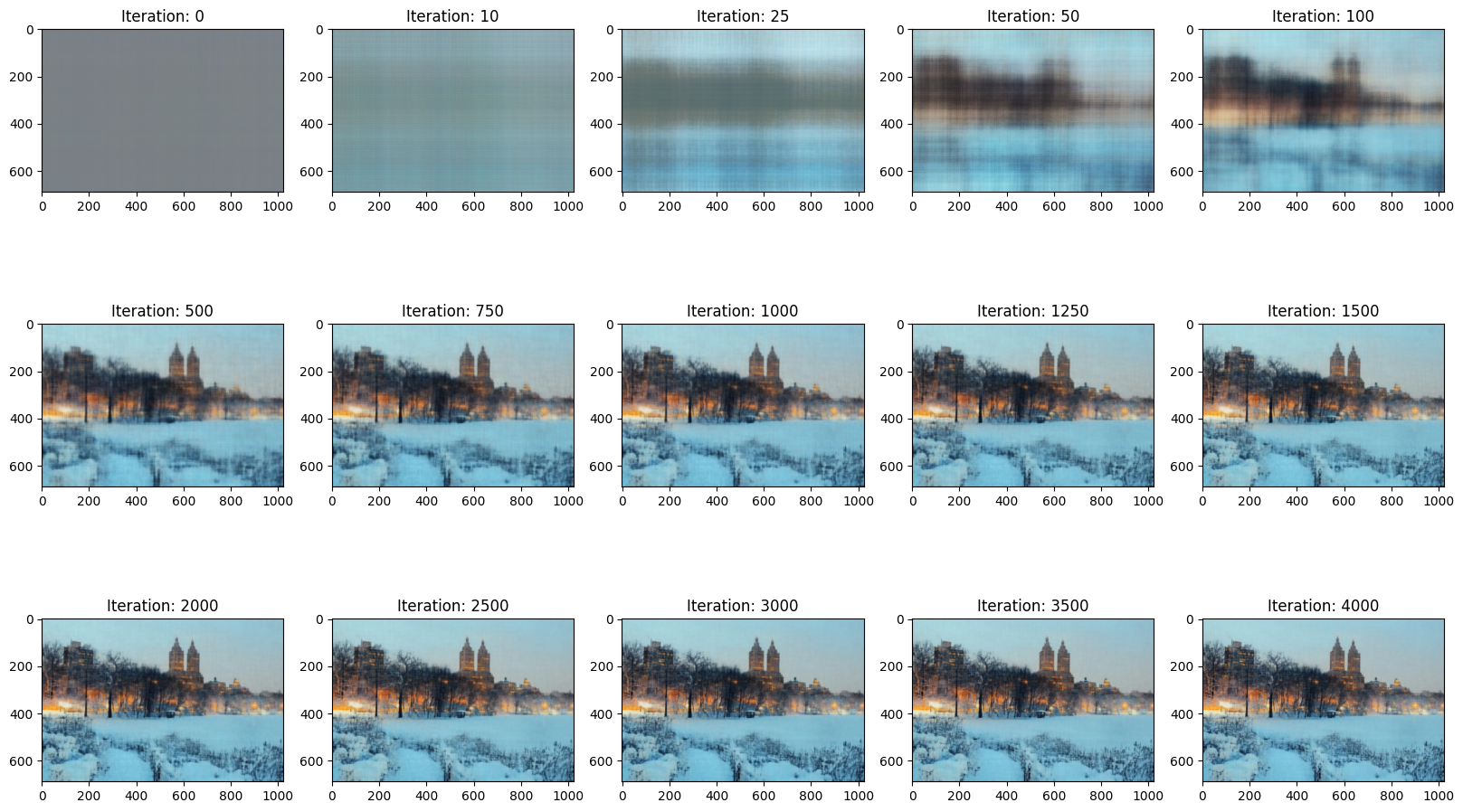
Before designing a multi-view neural radiance field, I implemented a neural radiance field in PyTorch to recreate an rgb image off of image coordinates with the below architecture. We first normalize our image and then apply positional encoding on the input layer of the network to deeply capture the spatial information of the coordinates. I used 4 hidden layers of initially 256 neurons each with ReLU activations in between and a final sigmoid activation. Lastly, I used Mean Squared Error to evaluate the loss and the Adam optimizer for gradient descent.
|
|
|
|
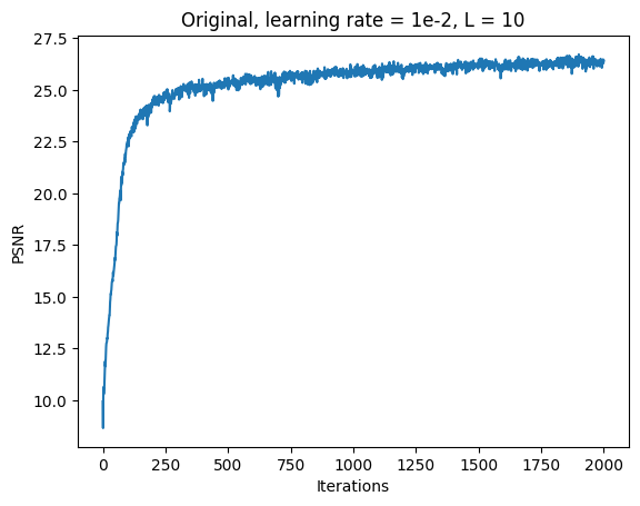
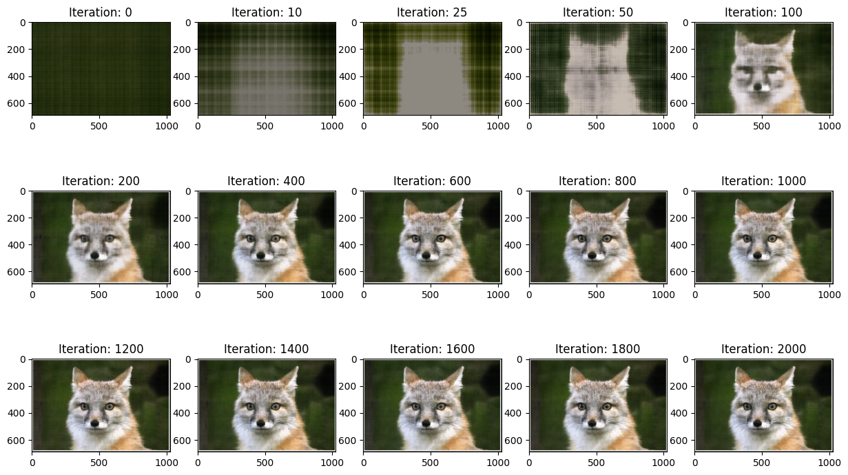
Original Fox Model 1: L = 10, Channel Size = 256, Learning Rate = 1e-2
|
|
Adjusting Learning Rate
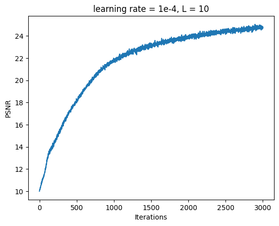
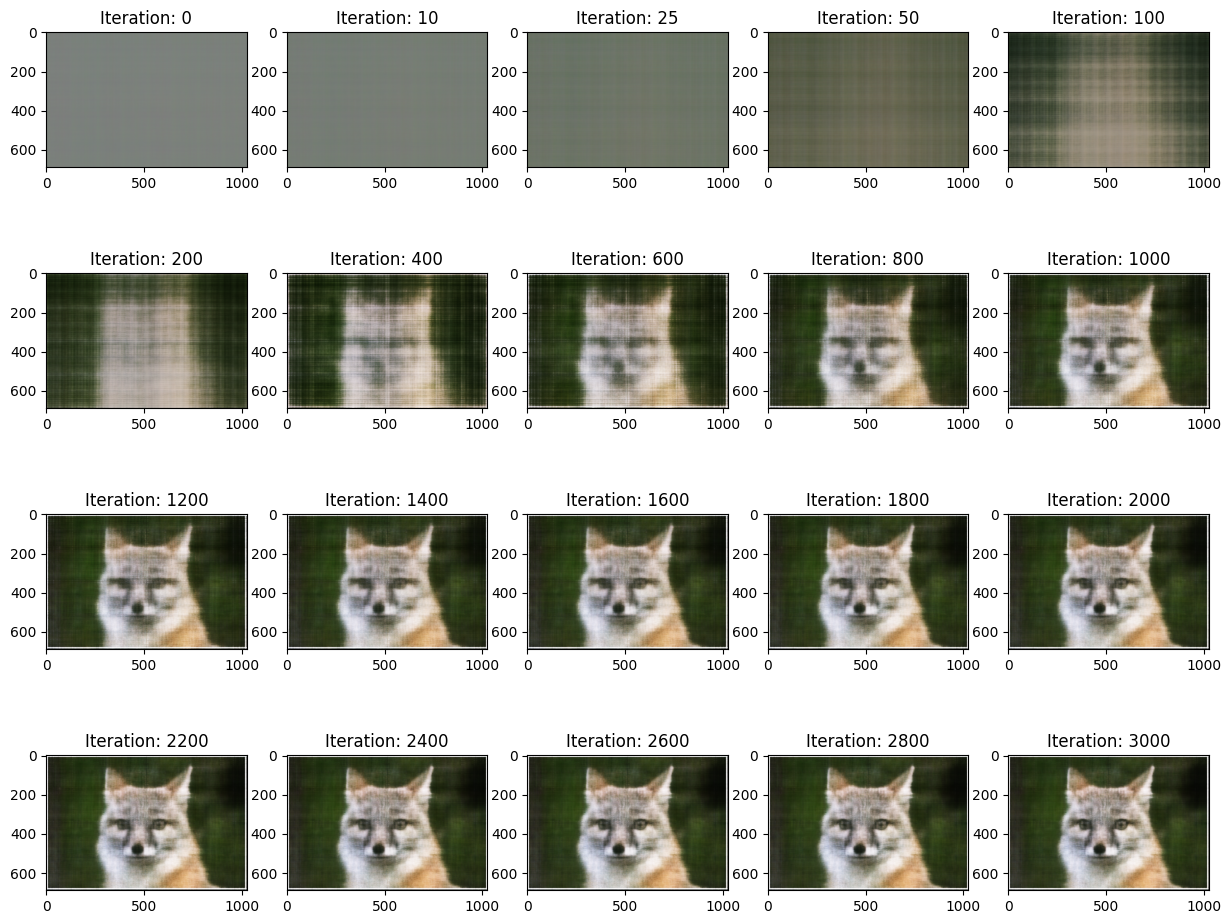
Fox Model 2A: L = 10, Channel Size = 256, Learning Rate = 1e-4
|
|
Reducing learning rate made model take longer to converge to the clear image.
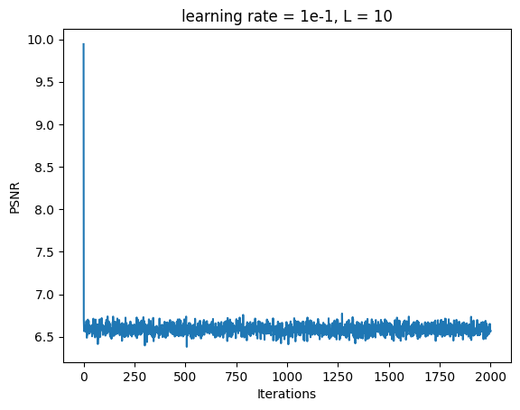
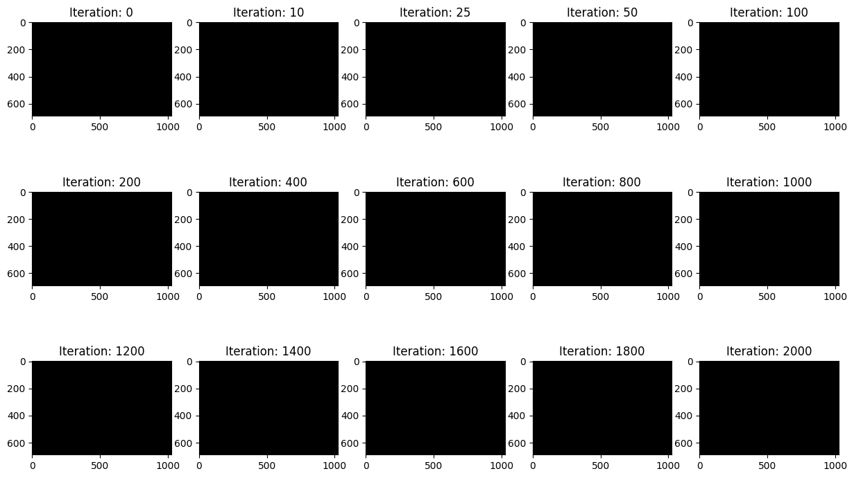
Fox Model 2B: L = 10, Channel Size = 256, Learning Rate = 1e-1
|
|
Increasing the learning rate prevented the model from learning
Adjusting Positional Encoding Length
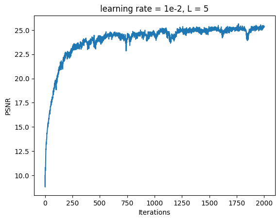
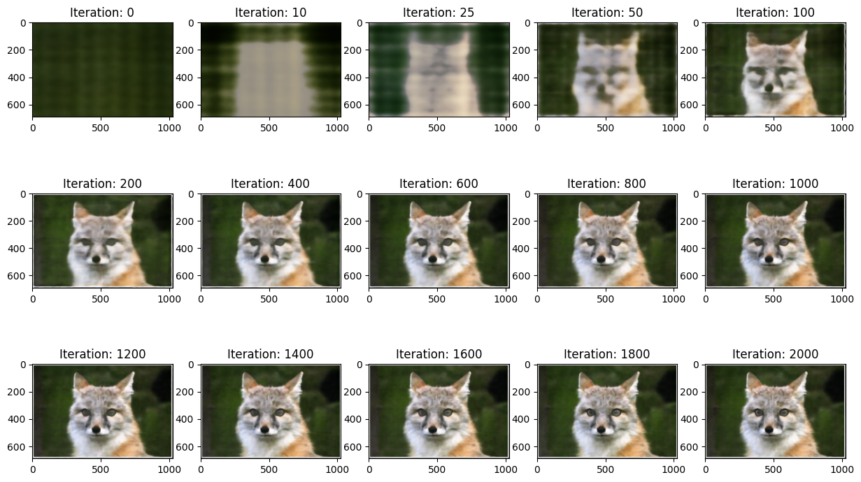
Fox Model 3A: L = 5, Channel Size = 256, Learning Rate = 1e-2
|
|
Decreasing the Positional Encoding length prevented the model from identifying high frequency features like the pupils of the fox.
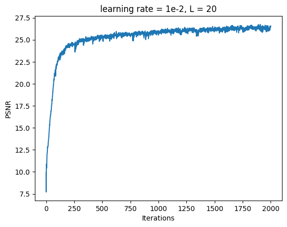
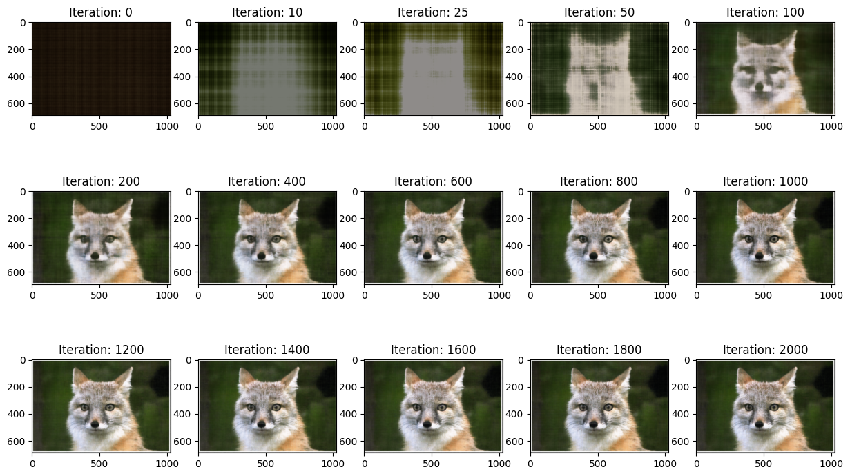
Fox Model 3B: L = 20, Channel Size = 256, Learning Rate = 1e-2
|
|
Increasing the Positional Encoding length had negligible differences compared to the default settings
|
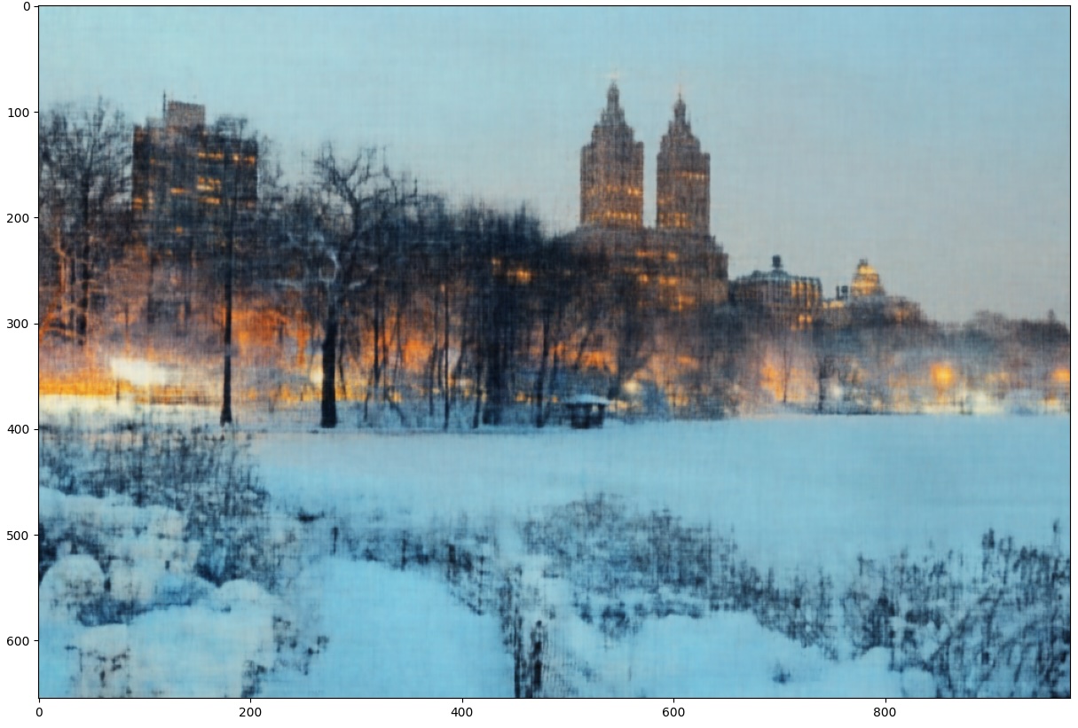
New York Model: L = 10, Channel Size = 256, Learning Rate = 1e-2, Total Iterations = 4000
|
|
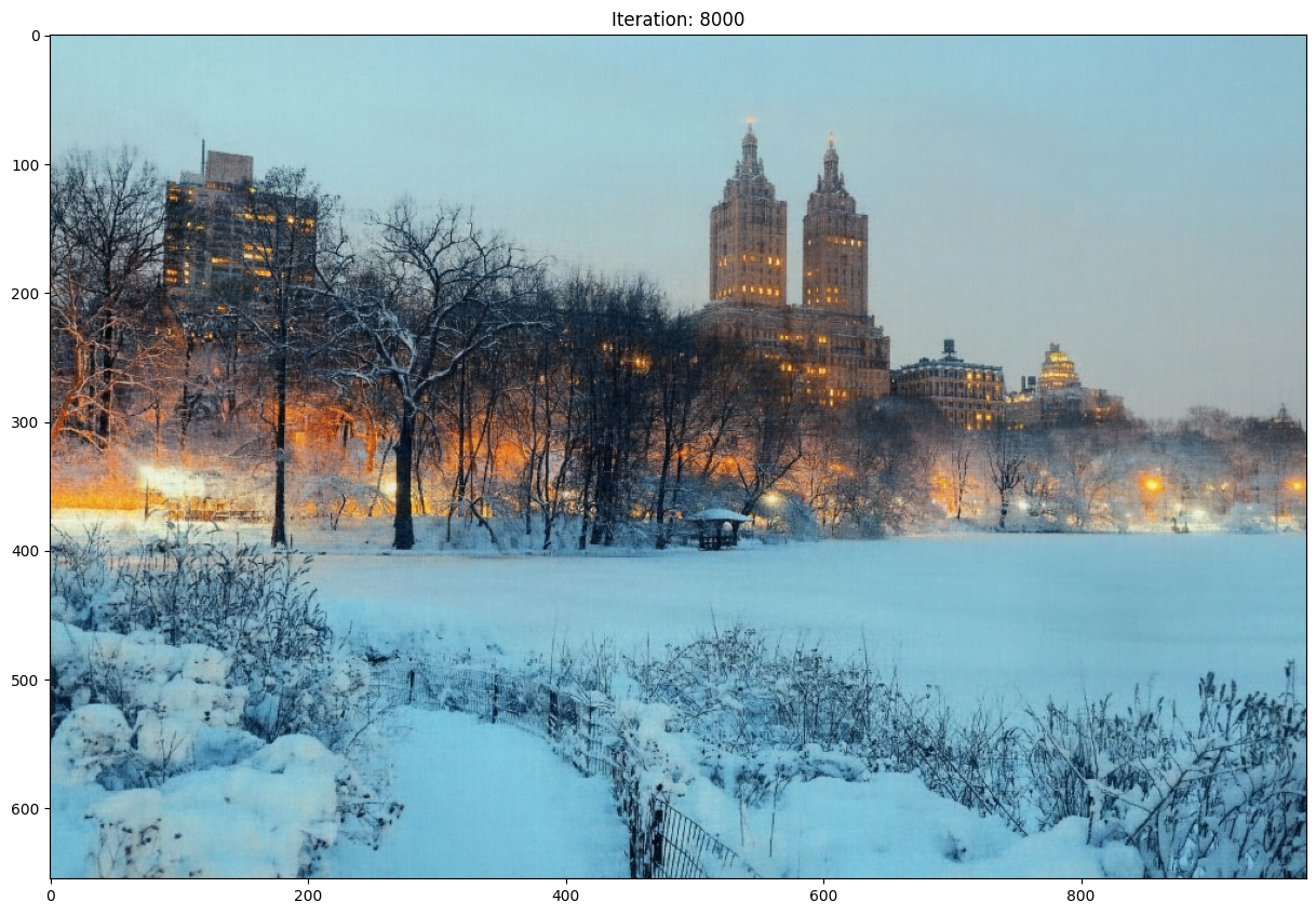
New York Model 2: L = 20, Channel Size = 768, Learning Rate = 0.0015, Total Iterations = 8000

|
|
 / /
|
|
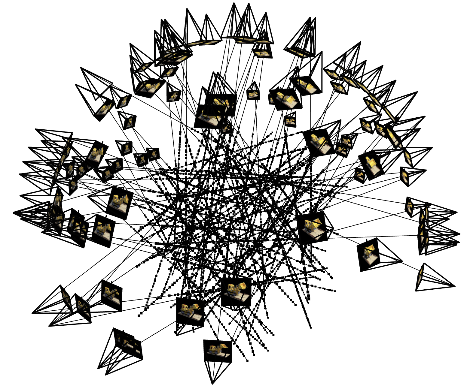
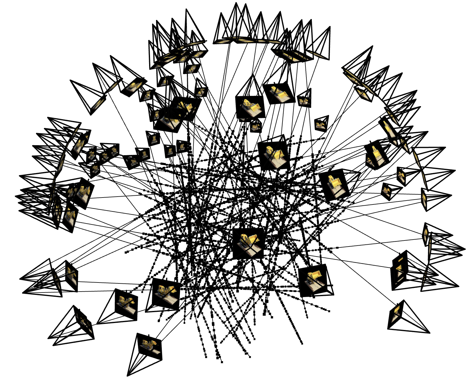
Ray Sampling
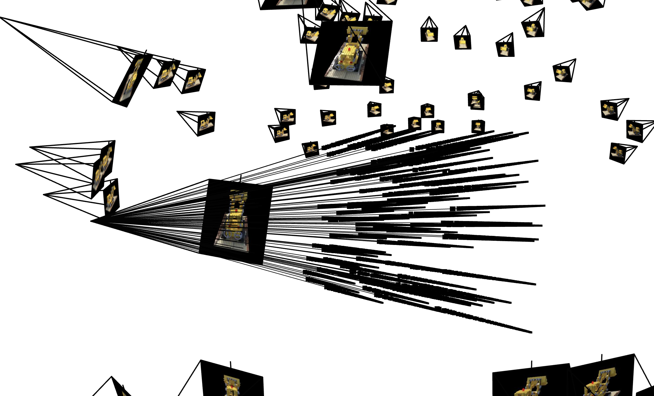
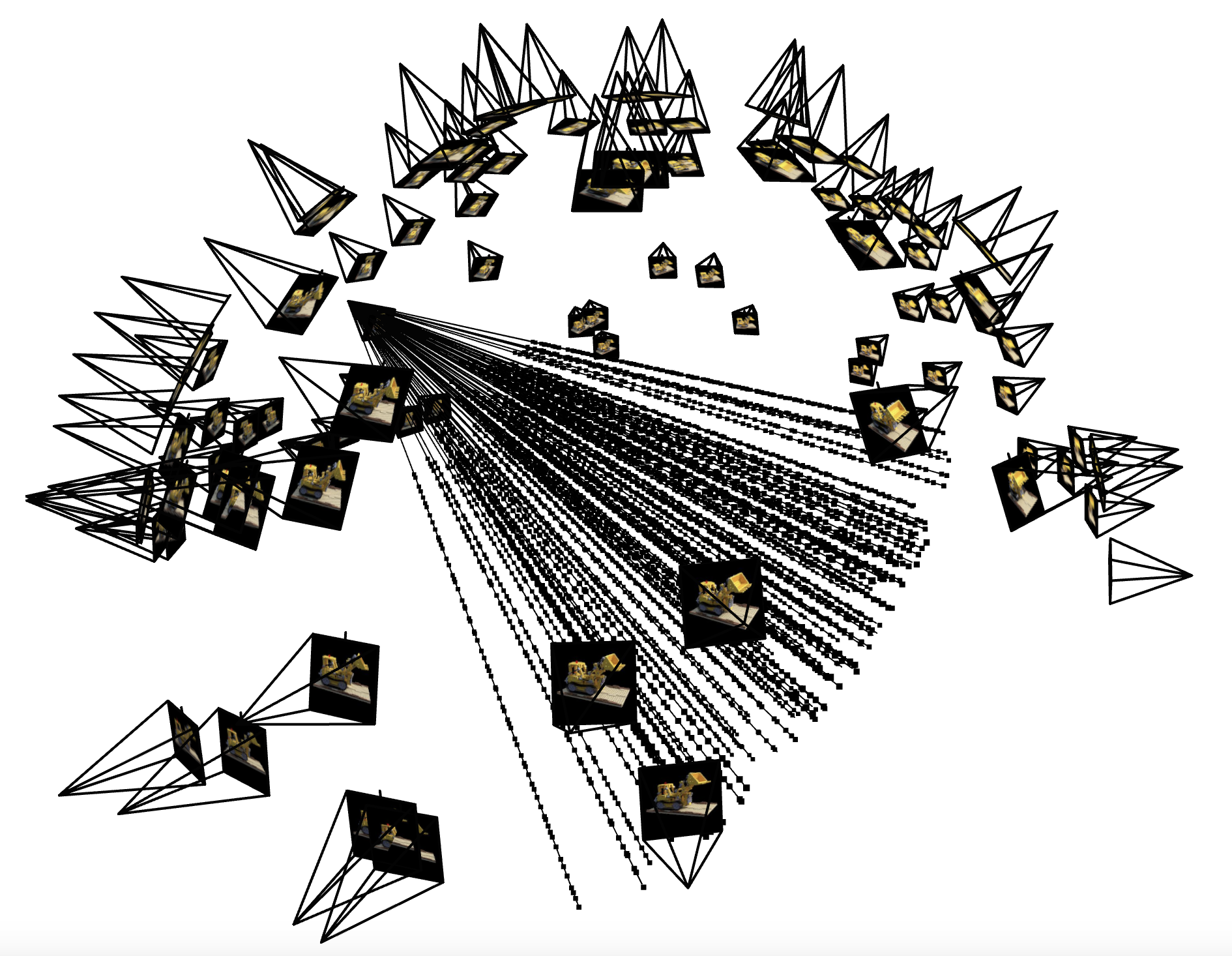
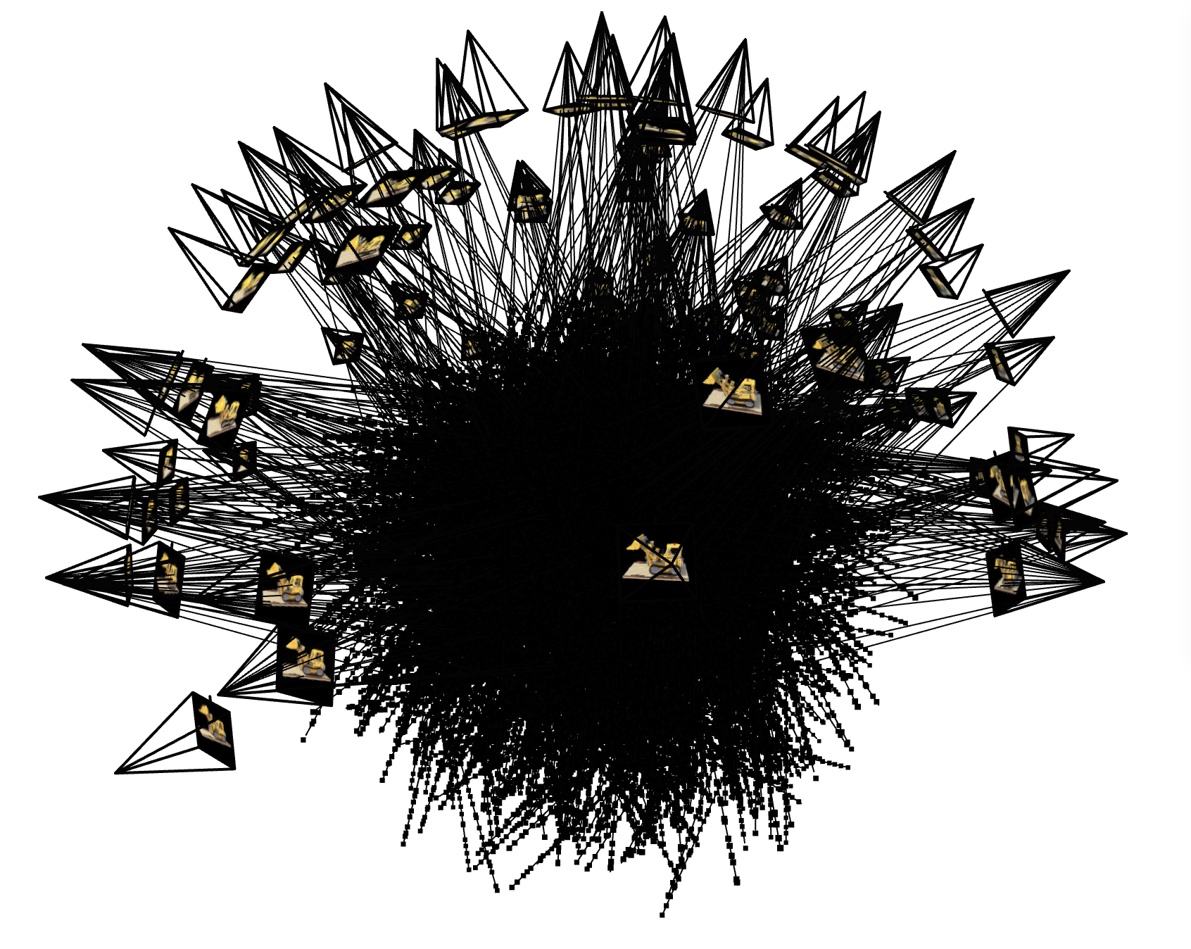
To collect our world space data, we first need to convert our image coordinates into rays, so we can pair our rays with pixel values later on. In order to do this, we first solve this problem for a single camera. We have to consider the setting in image space, camera space, and world space. We can generate samples of pixels easily in image space and then invert the intrinsic and extrinsic matrices of the camera in order to find where the pixel on the image would lie in world space.
We can use the camera's extrinsic matrix to similarly find where it exists in world space and with the world space locations of both the camera and the pixels, we can generate rays along these lines. We add noise to the samples to better generalize over the world space coordinates. The ray sampling results are visualized below.
|
|
|
|
|
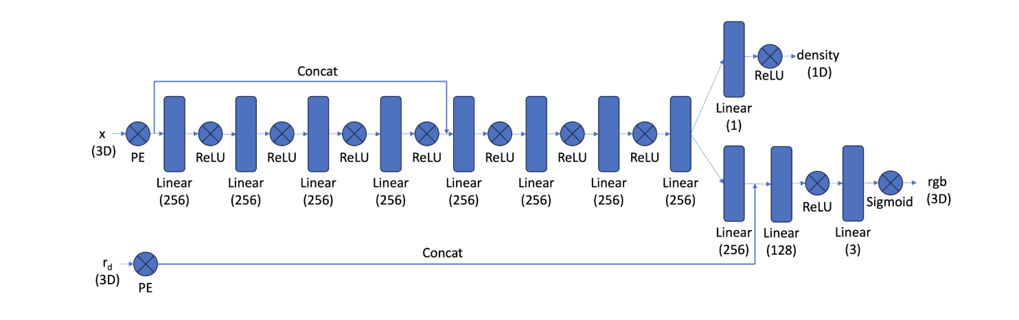
Neural Network Architecture
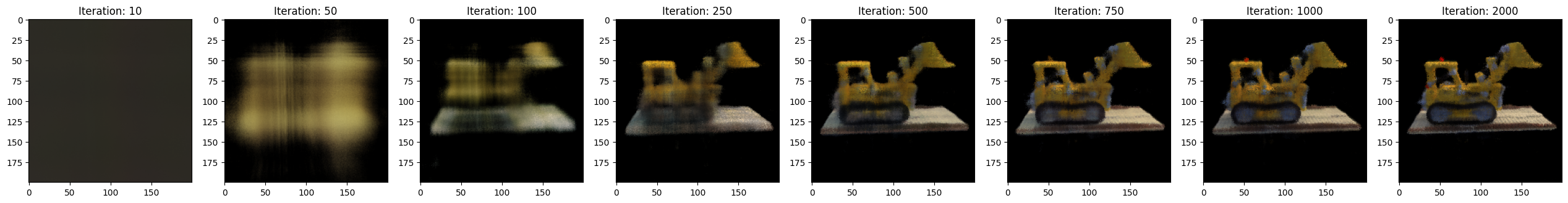
Here, we adjust the neural network to include inputs in both world coordinates and ray directions and output their rgb colors and densities. We utilize skip connections to ensure the spatial information is not forgotten in the 8+ layer network. To compute the predicted color of each ray, we use the volume rendering formula, which aggregates the color of each coordinate along the ray weighted by its density and the opacity of that point. We implemented volume rendering in a vectorized fashion in PyTorch to ensure it was differentiable for the loss function.
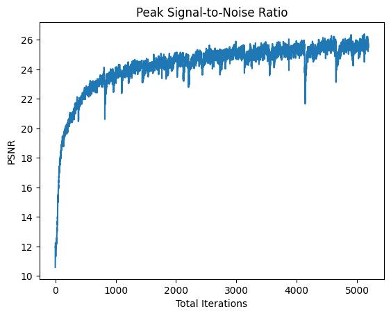
We compute this for every ray and in addition to the mean squared loss with the true pixel value from the image to backpropagate the error through the network. Here, we use a batch size of 10,000, a learning rate of 3e-3, and the Adam optimizer.
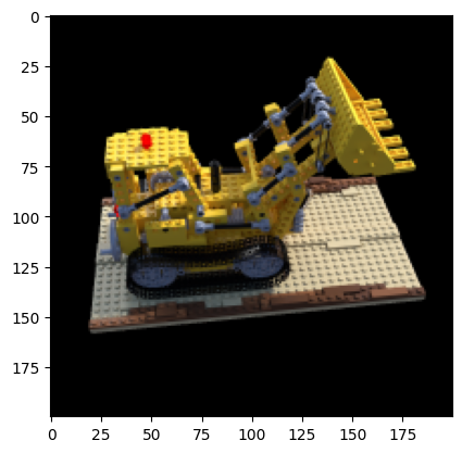
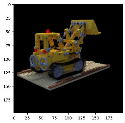
|
Training, Learning Rate = 2e-3,
|
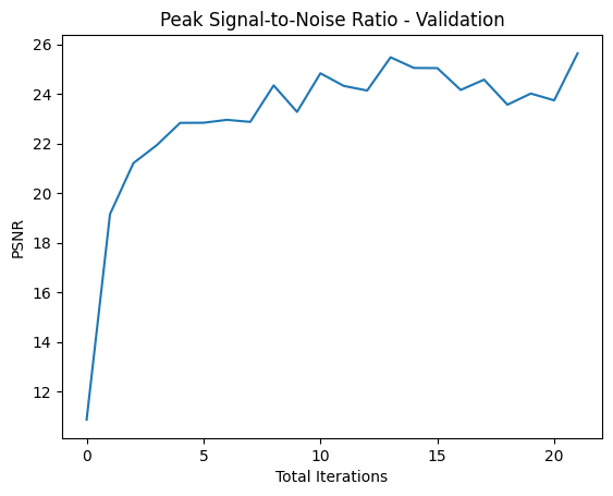
Validation
|
|
|
For depth, we use the same model to compute rgb values and densities for every ray. However, we switch out the rgb values with a gradient of white to black values from the camera to the end of the ray, while keeping the densities the same.
For background colors, I looked at the final element of the T array which carried the tranmittence of light at each point across the ray. If this value was high at the end of the ray, that would mean there aren't any dense objects in between so the ray would be generating the background. As a result, I looked for this component in each ray using torch.where() and if the T value was greater than a threshold (>0.999), I'd replace it with a bluish-green color, although the model still has some inaccuracies in some frames and around the edges.
|
|
|